Reinforcement Learning Rewards-based Algorithms - Primer
In reinforcement learning (RL), you learn what actions to take in a given environment to maximize cumulative rewards. In imitation learning (talked about in this post), the similarity between your action and the expert’s action in a given state guided the model on what action to take; in reinforcement learning, the rewards are what guides the model. In this post, I’m going to discuss how we can define this problem more concretely.
As a refresher, recall we can use Markov decision process (MDP) to describe a reinforcement learning problem and our policy’s goal is to maximize the total rewards.

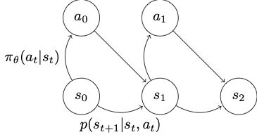
Let’s consider how our state transitions happen here given the policy. As shown in the diagram, your next state is determined by your last state and the action, and the action is determined by your policy; therefore, your single state transition can be expressed as \(\pi_\theta(a_t \vert s_t)p(s_{t+1} \vert s_{t},a_{t})\).
Then, the probability distribution of a trajectory \(\tau\) which consists of a sequence of state-action pairs is
\[p(\tau) = p(s_1)\prod^T_{t=1}\pi_\theta(a_t, s_t) p(s_{t+1} \vert s_t,a_t)\]The goal is to maximize the cumulative rewards over the trajectory; the learning objective is to find a policy such that it generates a trajectory that will give you the maximum rewards. The RL objective is
\[\mathop{\operatorname{arg\,max_\theta}} E_{\tau\sim p_\theta(\tau)} \sum_t r(s_t, a_t)\]Training Cycle
In supervised learning, since you are assuming data are independent, you can collect your data once and train your model against it multiple times.
In reinforcement learning, your policy (\(\pi\)), which action to take) and dynamics model (state transition, \(p(s_{t+1}\vert s_t,a_t)\)) are responsible for generating the future states that it predicts on. The data generation and learning are in a feedback loop. Therefore, we can’t simply do a single pass training (note that there is ample research going on in training reinforcement learning this way, called offline reinforcement learning); instead, RL methods run a multiple cycles of the following:
- generate samples \((s,a)\). In this step, you run roll out your policy; if you need to bootstrap, you might prepare some expert data.
- fit a dynamics model model (\(p(s_{t+1}\vert s_t,a_t)\)) or estimate the total rewards (\(E(r)\))
- improve the policy
There are a few options you can use in step 2 and 3. The first distinction I will note is model-based vs. model-free.
Model-based vs Model-free Learning
Going back to the markov diagram, we can say the probability distribution of a rollout is \(p(s_1)\prod^T_{t=1}\pi_\theta(a_t, s_t) p(s_{t+1} \vert s_t,a_t)\).
In the model-free approach, we do not try to learn \(p(s_{t+1}\vert s_t,a_t)\) or estimate the rewards; instead we directly observe the outcome of the policy and focus on fitting the policy.
In the model-based approach, we try to learn the system dynamics. For example, suppose we are building a robot that can pick up an object from one place and drop it in another place; in model-based reinforcement learning, we will have an understanding of where the robot arm will be (\(s_{t+1}\)) after it has moved its arm right once (\(a_t\)) from where it was (\(s_t\)). A robot running per policy trained by a model-free RL method will take actions with the expectation of higher rewards, but will not be able to predict what the resulting state will be from its actions.
Both approaches have been shown to work in different problems; they are both potentially great ways of solving more and more intelligent problems in AI.
In the next few posts, we will discuss a few options within model-free approach, starting from policy gradient.